On the other hand
Internet home of C. Susannah Tysor
The Commons
In an era when biomedical research[1] is becoming increasingly digital and analytical, the current support system is neither cost-effective nor sustainable. Moreover, that digital content is hard to find and use. The Commons is a pilot experiment in the efficient storage, manipulation, analysis, and sharing of research output, from all parts of the research lifecycle. Should The Commons be successful we would achieve a level of comprehensive access and interoperability across the research enterprise far beyond what is possible today.
The Commons is a conceptual framework for a digital environment to allow efficient storage, manipulation, and sharing of research objects[2].
My ugly pet
Every time my code spit out an error or didn’t work properly, I felt like I was idiot – that the computer was “right” and I was “wrong.”
This is extremely unhelpful, but I’m not the only one to have this reaction while learning programming.
There’s this saying that computers only do what you tell them to do. So if you get an error, you must have told the computer to do something wrong. After all, the computer is a precise machine of perfect logic, right?
What freed me from my counterproductive response to errors was realizing that I am not laying my code at the alter of some sort of perfect mathematical god and asking for their blessing. I realized that I’m working with things that other people made with a variety of goals and constraints.
A programming language implementation is itself a program. Features of that program may have been fought over, made on deadlines, meant to be fixed later, a joke, a personal preference, or just not that well understood. The rules of a programming language interact in complex ways that can be hard to foresee, even for the designers, and the interpreters and compilers that implement those rules may also have bugs of their own.
So when you come along and try to write your code in that language, you may get all kinds of weird and terrible and surprising effects. You can, with work and good documentation, usually figure out a bug, but a programming language is more like a very ugly pet that can do very cool tricks than a system of perfect sense and logic.
I don’t worry about being wrong so much anymore. Instead I think “how do I get this strange beast to behave the way I want it to?”
Projecting a map to match your data in R
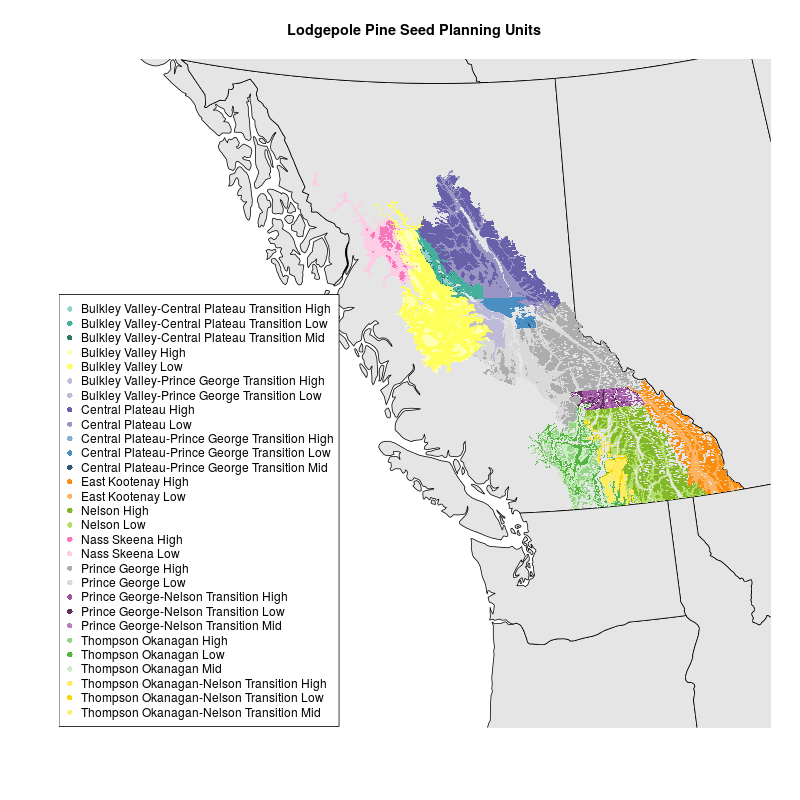
I had a shapefile of lodgepole pine seed planning units (SPUs) in the BC Environment Standard Projection, which is an Albers Equal Area Conic projection with specific parameters. I tried creating a map with mapproject in R as explained by Kim Gilbert. I used an Albers projection with the parameters described here and in the .prj file associated with my data . But I couldn’t get the map of Western Canada and the shapefile of SPUs to plot together. I’m not sure why.
I took a different approach based on this StackExchange GIS question. I downloaded a shapefile for the world, projected it using rgdal::spTransform, clipped it to the extent I was interested in, and mapped it with the SPU shapefile. Map and code are below. Data for SPUs is not included.
library(rgdal)

# Get basemap data
download.file(url="http://www.naturalearthdata.com/http//www.naturalearthdata.com/download/50m/cultural/ne_50m_admin_1_states_provinces.zip", "ne_50m_admin_1_states_provinces.zip", "auto")
unzip("ne_50m_admin_1_states_provinces.zip")
file.remove("ne_50m_admin_1_states_provinces.zip")

# read basemap shape file using rgdal library
ogrInfo(".", "ne_50m_admin_1_states_provinces_shp")
world <- readOGR(".", "ne_50m_admin_1_states_provinces_shp")
summary(world)

#project basemap to match spu shapefile
worldBCESP <- spTransform(world, CRS("+proj=aea +lat_1=50 +lat_2=58.5 +lat_0=45 +lon_0=-126 +x_0=1000000 +y_0=0 +ellps=GRS80 +datum=NAD83 +units=m +no_defs")) #proj4 string from http://spatialreference.org/ref/sr-org/82/
summary(worldBCESP)

#make color palette for SPUS
palette(c("#8DD3C7", "#45B09E", "#2E766A",
          "#FFFFB3", "#FFFF5C",
        "#BEBADA", "#BEBADA",
        "#6860A9", "#9B95C6",
        "#80B1D3", "#498FC1", "#2A587A",
        "#FB8D0E", "#FDB462",
        "#83B828", "#B3DE69",
        "#F778BA", "#FCCDE5",
        "#ADADAD", "#D9D9D9",
        "#A053A2", "#5D315E", "#BC80BD",
        "#94D585", "#54B63E", "#CCEBC5",
        "#FFEC5C", "#F5D800", "#FFED6F"))

# Read in shapefile for SPUs
spu <- readOGR("maps/SPUmaps/SPU_Tongli", layer="Pli_SPU")
levels(spu$SPU) <- c("Bulkley Valley-Central Plateau Transition High", "Bulkley Valley-Central Plateau Transition Low", "Bulkley Valley-Central Plateau Transition Mid", "Bulkley Valley High", "Bulkley Valley Low", "Bulkley Valley-Prince George Transition High", "Bulkley Valley-Prince George Transition Low", "Central Plateau High", "Central Plateau Low", "Central Plateau-Prince George Transition High", "Central Plateau-Prince George Transition Low", "Central Plateau-Prince George Transition Mid", "East Kootenay High", "East Kootenay Low", "Nelson High", "Nelson Low", "Nass Skeena High", "Nass Skeena Low", "Prince George High", "Prince George Low", "Prince George-Nelson Transition High", "Prince George-Nelson Transition Low", "Prince George-Nelson Transition Mid", "Thompson Okanagan High", "Thompson Okanagan Low", "Thompson Okanagan Mid", "Thompson Okanagan-Nelson Transition High", "Thompson Okanagan-Nelson Transition Low", "Thompson Okanagan-Nelson Transition Mid") #make levels human readable


#make plot
png("SPUmap.png", width=800, height=800)

plot(worldBCESP, xlim=c(0,1870556), ylim=c(157057.2,1421478), col="gray90") #plot basemap
plot(spu, add=TRUE, border=FALSE, col=spu$SPU) #plot SPUs
legend('bottomleft', legend = levels(spu$SPU), col = 1:length(levels(spu$SPU)), cex = 1, pch = 16) #plot legend
title("Lodgepole Pine Seed Planning Units")

dev.off()
