… I came to see the owls as one of countless shapes the forest assumes, more than as an animal that resides in a forest. In this view, if the organism is removed from the old growth, it ceases to be a spotted owl and becomes just a brown, speckled, dark-eyed, meat-eating bird.
The feature that most exemplifies this awareness for me is the owl’s feathers. Unlike most raptors in this region, northern spotted owls don’t migrate south in the winter. They are here in rain and snow and cold. Yet they are not exceptional thermoregulators as one would expect of a nonmigrant facing a rainy, snowy Cascade Mountain winter.
The reason for this counterintuitive disparity is the old-growth forest, which buffers temperature extremes at both ends of the spectrum by as much as twenty degrees Fahrenheit in relation to adjacent clearings. The owls wear old growth like another layer of feathers. That is, their preferred habitat provides sufficient thermal protection, so that they do not have to expend energy growing as much down as they would need if they dwelled in open country.
The deep multilayered canopy characteristic of old-growth groves also intercepts enough snow to permit the owl’s preferred prey species – the northern flying squirrel – to remain active all winter long, feeding on truffle mushrooms on the open ground at the bottom of snow wells around the bases of the trees. With food and warmth (as well as many other life needs) literally covered by the old growth, the owl does not have to make a long flight to warmer climes at the onset of autumn.
Instead, the owl makes short flights in response to immediate conditions. Sun gaps on otherwise snowy January days draw them out from beneath sheltering midcanopy mistletoe umbrellas to ascend to high branches, where direct solar radiance can offer springlike warmth even during the coldest time of year. And in the heat of August, the owls are often found perched low in vine maples a few feet above a cooling creek in shady northeast- facing drainages. This behavioural thermoregulation and the incorporation of the forest itself into their meaningful physiology provide just two of many possible examples that demonstrate why efforts to reduce the spotted owl to a bird in a habitat represents extreme oversimplification.
from The Mountain Lion by Tim Fox, excerpted in Forest Under Story
On the other hand
Internet home of C. Susannah Tysor
Category Archives: Uncategorized
The Commons
In an era when biomedical research[1] is becoming increasingly digital and analytical, the current support system is neither cost-effective nor sustainable. Moreover, that digital content is hard to find and use. The Commons is a pilot experiment in the efficient storage, manipulation, analysis, and sharing of research output, from all parts of the research lifecycle. Should The Commons be successful we would achieve a level of comprehensive access and interoperability across the research enterprise far beyond what is possible today.
The Commons is a conceptual framework for a digital environment to allow efficient storage, manipulation, and sharing of research objects[2].
Projecting a map to match your data in R
I had a shapefile of lodgepole pine seed planning units (SPUs) in the BC Environment Standard Projection, which is an Albers Equal Area Conic projection with specific parameters. I tried creating a map with mapproject in R as explained by Kim Gilbert. I used an Albers projection with the parameters described here and in the .prj file associated with my data . But I couldn’t get the map of Western Canada and the shapefile of SPUs to plot together. I’m not sure why.
I took a different approach based on this StackExchange GIS question. I downloaded a shapefile for the world, projected it using rgdal::spTransform, clipped it to the extent I was interested in, and mapped it with the SPU shapefile. Map and code are below. Data for SPUs is not included.
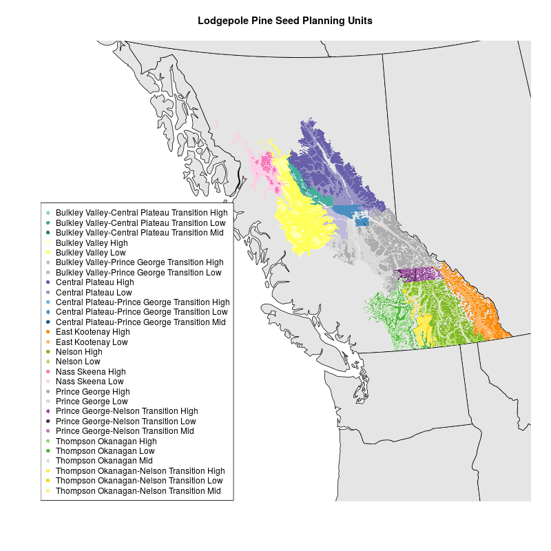
Map of Lodgepole Pine by Susannah Tysor in R with data from Tongli Wang
library(rgdal)

# Get basemap data
download.file(url="http://www.naturalearthdata.com/http//www.naturalearthdata.com/download/50m/cultural/ne_50m_admin_1_states_provinces.zip", "ne_50m_admin_1_states_provinces.zip", "auto")
unzip("ne_50m_admin_1_states_provinces.zip")
file.remove("ne_50m_admin_1_states_provinces.zip")

# read basemap shape file using rgdal library
ogrInfo(".", "ne_50m_admin_1_states_provinces_shp")
world <- readOGR(".", "ne_50m_admin_1_states_provinces_shp")
summary(world)

#project basemap to match spu shapefile
worldBCESP <- spTransform(world, CRS("+proj=aea +lat_1=50 +lat_2=58.5 +lat_0=45 +lon_0=-126 +x_0=1000000 +y_0=0 +ellps=GRS80 +datum=NAD83 +units=m +no_defs")) #proj4 string from http://spatialreference.org/ref/sr-org/82/
summary(worldBCESP)

#make color palette for SPUS
palette(c("#8DD3C7", "#45B09E", "#2E766A",
          "#FFFFB3", "#FFFF5C",
        "#BEBADA", "#BEBADA",
        "#6860A9", "#9B95C6",
        "#80B1D3", "#498FC1", "#2A587A",
        "#FB8D0E", "#FDB462",
        "#83B828", "#B3DE69",
        "#F778BA", "#FCCDE5",
        "#ADADAD", "#D9D9D9",
        "#A053A2", "#5D315E", "#BC80BD",
        "#94D585", "#54B63E", "#CCEBC5",
        "#FFEC5C", "#F5D800", "#FFED6F"))

# Read in shapefile for SPUs
spu <- readOGR("maps/SPUmaps/SPU_Tongli", layer="Pli_SPU")
levels(spu$SPU) <- c("Bulkley Valley-Central Plateau Transition High", "Bulkley Valley-Central Plateau Transition Low", "Bulkley Valley-Central Plateau Transition Mid", "Bulkley Valley High", "Bulkley Valley Low", "Bulkley Valley-Prince George Transition High", "Bulkley Valley-Prince George Transition Low", "Central Plateau High", "Central Plateau Low", "Central Plateau-Prince George Transition High", "Central Plateau-Prince George Transition Low", "Central Plateau-Prince George Transition Mid", "East Kootenay High", "East Kootenay Low", "Nelson High", "Nelson Low", "Nass Skeena High", "Nass Skeena Low", "Prince George High", "Prince George Low", "Prince George-Nelson Transition High", "Prince George-Nelson Transition Low", "Prince George-Nelson Transition Mid", "Thompson Okanagan High", "Thompson Okanagan Low", "Thompson Okanagan Mid", "Thompson Okanagan-Nelson Transition High", "Thompson Okanagan-Nelson Transition Low", "Thompson Okanagan-Nelson Transition Mid") #make levels human readable


#make plot
png("SPUmap.png", width=800, height=800)

plot(worldBCESP, xlim=c(0,1870556), ylim=c(157057.2,1421478), col="gray90") #plot basemap
plot(spu, add=TRUE, border=FALSE, col=spu$SPU) #plot SPUs
legend('bottomleft', legend = levels(spu$SPU), col = 1:length(levels(spu$SPU)), cex = 1, pch = 16) #plot legend
title("Lodgepole Pine Seed Planning Units")

dev.off()