I had a shapefile of lodgepole pine seed planning units (SPUs) in the BC Environment Standard Projection, which is an Albers Equal Area Conic projection with specific parameters. I tried creating a map with mapproject in R as explained by Kim Gilbert. I used an Albers projection with the parameters described here and in the .prj file associated with my data . But I couldn’t get the map of Western Canada and the shapefile of SPUs to plot together. I’m not sure why.
I took a different approach based on this StackExchange GIS question. I downloaded a shapefile for the world, projected it using rgdal::spTransform, clipped it to the extent I was interested in, and mapped it with the SPU shapefile. Map and code are below. Data for SPUs is not included.
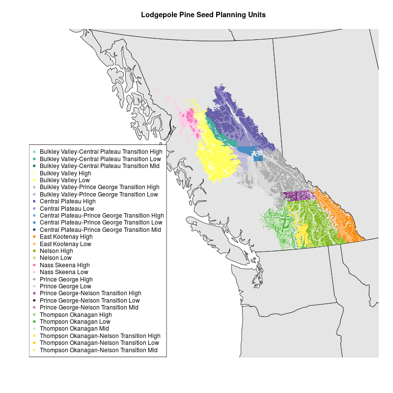
Map of Lodgepole Pine by Susannah Tysor in R with data from Tongli Wang
library(rgdal)

# Get basemap data
download.file(url="http://www.naturalearthdata.com/http//www.naturalearthdata.com/download/50m/cultural/ne_50m_admin_1_states_provinces.zip", "ne_50m_admin_1_states_provinces.zip", "auto")
unzip("ne_50m_admin_1_states_provinces.zip")
file.remove("ne_50m_admin_1_states_provinces.zip")

# read basemap shape file using rgdal library
ogrInfo(".", "ne_50m_admin_1_states_provinces_shp")
world <- readOGR(".", "ne_50m_admin_1_states_provinces_shp")
summary(world)

#project basemap to match spu shapefile
worldBCESP <- spTransform(world, CRS("+proj=aea +lat_1=50 +lat_2=58.5 +lat_0=45 +lon_0=-126 +x_0=1000000 +y_0=0 +ellps=GRS80 +datum=NAD83 +units=m +no_defs")) #proj4 string from http://spatialreference.org/ref/sr-org/82/
summary(worldBCESP)

#make color palette for SPUS
palette(c("#8DD3C7", "#45B09E", "#2E766A",
          "#FFFFB3", "#FFFF5C",
        "#BEBADA", "#BEBADA",
        "#6860A9", "#9B95C6",
        "#80B1D3", "#498FC1", "#2A587A",
        "#FB8D0E", "#FDB462",
        "#83B828", "#B3DE69",
        "#F778BA", "#FCCDE5",
        "#ADADAD", "#D9D9D9",
        "#A053A2", "#5D315E", "#BC80BD",
        "#94D585", "#54B63E", "#CCEBC5",
        "#FFEC5C", "#F5D800", "#FFED6F"))

# Read in shapefile for SPUs
spu <- readOGR("maps/SPUmaps/SPU_Tongli", layer="Pli_SPU")
levels(spu$SPU) <- c("Bulkley Valley-Central Plateau Transition High", "Bulkley Valley-Central Plateau Transition Low", "Bulkley Valley-Central Plateau Transition Mid", "Bulkley Valley High", "Bulkley Valley Low", "Bulkley Valley-Prince George Transition High", "Bulkley Valley-Prince George Transition Low", "Central Plateau High", "Central Plateau Low", "Central Plateau-Prince George Transition High", "Central Plateau-Prince George Transition Low", "Central Plateau-Prince George Transition Mid", "East Kootenay High", "East Kootenay Low", "Nelson High", "Nelson Low", "Nass Skeena High", "Nass Skeena Low", "Prince George High", "Prince George Low", "Prince George-Nelson Transition High", "Prince George-Nelson Transition Low", "Prince George-Nelson Transition Mid", "Thompson Okanagan High", "Thompson Okanagan Low", "Thompson Okanagan Mid", "Thompson Okanagan-Nelson Transition High", "Thompson Okanagan-Nelson Transition Low", "Thompson Okanagan-Nelson Transition Mid") #make levels human readable


#make plot
png("SPUmap.png", width=800, height=800)

plot(worldBCESP, xlim=c(0,1870556), ylim=c(157057.2,1421478), col="gray90") #plot basemap
plot(spu, add=TRUE, border=FALSE, col=spu$SPU) #plot SPUs
legend('bottomleft', legend = levels(spu$SPU), col = 1:length(levels(spu$SPU)), cex = 1, pch = 16) #plot legend
title("Lodgepole Pine Seed Planning Units")

dev.off()