I made a map in R for the first time last week using these guides by Kim Gilbert and Mollie Taylor.
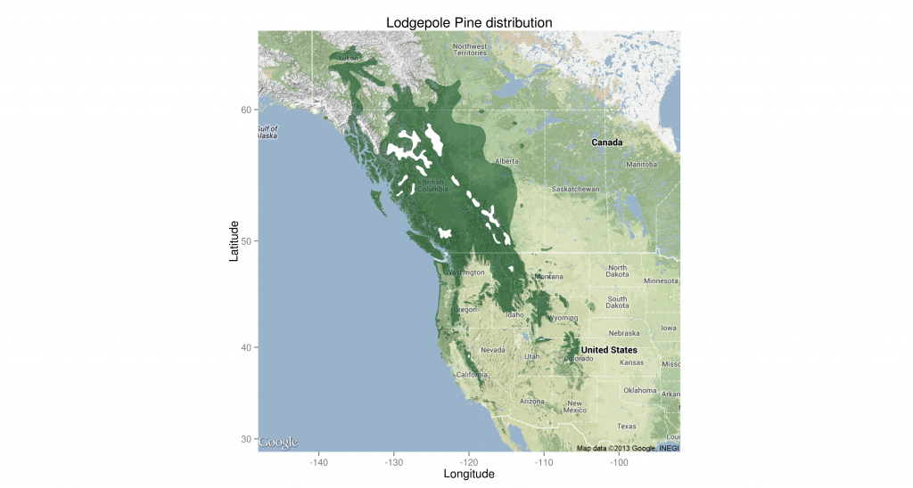
Pinus contorta range map including all subspecies. White areas within the distribution boundary contain no lodgepole. Based on Little 1971.
As you can see, I wasn’t able to show the holes in the distribution properly. Ideally, they would be actual holes showing the base map. I couldn’t get geom_map to not fill in the holes, so I overfilled them with white.
The code for the map is below and the shapefile I used is from the USGS GECSC Tree Species Distribution Maps for North America.
If anyone’s got a shapefile for just subspecies latifolia or a more recent distribution map, I’d love to use it.
pcontorta <- readShapePoly("pinucont.shp")
colors <- brewer.pal(9, "BuGn") # make pretty color palette

basemap <- get_map(location = c(lon = -120, lat= 50), #build basemap of Western North America
  color = 'color',
  source = 'google',
  maptype = 'terrain',
  zoom = 4)
basemap <- ggmap(basemap)

pcontorta.points <- fortify(pcontorta)

lodgepole <- geom_map(inherit.aes = FALSE, #make a layer for the lodgepole distribution
  aes(map_id=id),
  data=pcontorta.points,
  map=pcontorta.points,
  fill = colors[9],
  alpha = .5 )

holes <- geom_map(inherit.aes = FALSE, #fill the holes with white
  aes(map_id=id),
  data = pcontorta.points[which(pcontorta.points$hole==TRUE),],
  map=pcontorta.points[which(pcontorta.points$hole==TRUE),],
  fill = "#FFFFFF",
  alpha = 1 )

basemap + lodgepole + holes + #put it all together
xlab("Longitude") + ylab("Latitude") +
ggtitle("Lodgepole Pine distribution")
