Category Archives: Computery

Problems setting root.dir in knitr

RStudio sets the working directory to the project directory, but knitr sets the working directory to the .Rmd file directory. This creates issues when you are sourcing files relative to the project directory in your R markdown file. Specifically, knitr tells you it can’t find those files:

Error in file(filename, "r", encoding = encoding) : 
  cannot open the connection
In addition: Warning message:
In file(filename, "r", encoding = encoding) :
  cannot open file 'home/sus/Documents/research_phd/analysis/phenodata_explore.R': No such file or directory

knitr has an option for dealing with this – root.dir – and Phil Mike Jones even gives a nice little knitr chunk example of using it.

But when I tried it, knitr kept failing to find my file.

```{r "setup", include=FALSE}
require("knitr")
opts_knit$set(root.dir = "~/Documents/research_phd/")
source('analysis/someanalysis.R')
```

It turns out I should have read the documentation more closely.

Knitr’s settings must be set in a chunk before any chunks which rely on those settings to be active. It is recommended to create a knit configuration chunk as the first chunk in a script with cache = FALSE and include = FALSE options set. This chunk must not contain any commands which expect the settings in the configuration chunk to be in effect at the time of execution.

Breaking it into two chunks separating the knitr configuration from the sourcing solved the problem.

```{r "knitr config", cache = FALSE, include=FALSE}
require("knitr")
opts_knit$set(root.dir = "~/Documents/research_phd/")
```

```{r, "setup", echo = FALSE}
source('analysis/someanalysis.R')
```
Tagged

My ugly pet

Every time my code spit out an error or didn’t work properly, I felt like I was idiot – that the computer was “right” and I was “wrong.”

This is extremely unhelpful, but I’m not the only one to have this reaction while learning programming.

There’s this saying that computers only do what you tell them to do. So if you get an error, you must have told the computer to do something wrong. After all, the computer is a precise machine of perfect logic, right?

What freed me from my counterproductive response to errors was realizing that I am not laying my code at the alter of some sort of perfect mathematical god and asking for their blessing. I realized that I’m working with things that other people made with a variety of goals and constraints.

A programming language implementation is itself a program. Features of that program may have been fought over, made on deadlines, meant to be fixed later, a joke, a personal preference, or just not that well understood. The rules of a programming language interact in complex ways that can be hard to foresee, even for the designers, and the interpreters and compilers that implement those rules may also have bugs of their own.

So when you come along and try to write your code in that language, you may get all kinds of weird and terrible and surprising effects. You can, with work and good documentation, usually figure out a bug, but a programming language is more like a very ugly pet that can do very cool tricks than a system of perfect sense and logic.

I don’t worry about being wrong so much anymore. Instead I think “how do I get this strange beast to behave the way I want it to?”

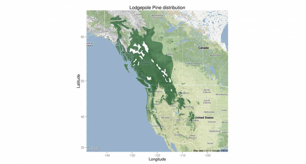
Pinus contorta distribution map in #rstats

I made a map in R for the first time last week using these guides by Kim Gilbert and Mollie Taylor.

Pinus contorta range map including all subspecies. White areas within the distribution boundary contain no lodgepole. Based on Little 1971.

Pinus contorta range map including all subspecies. White areas within the distribution boundary contain no lodgepole. Based on Little 1971.

As you can see, I wasn’t able to show the holes in the distribution properly. Ideally, they would be actual holes showing the base map. I couldn’t get geom_map to not fill in the holes, so I overfilled them with white.

The code for the map is below and the shapefile I used is from the USGS GECSC Tree Species Distribution Maps for North America.

If anyone’s got a shapefile for just subspecies latifolia or a more recent distribution map, I’d love to use it.

pcontorta <- readShapePoly("pinucont.shp")
colors <- brewer.pal(9, "BuGn") # make pretty color palette

basemap <- get_map(location = c(lon = -120, lat= 50), #build basemap of Western North America
  color = 'color',
  source = 'google',
  maptype = 'terrain',
  zoom = 4)
basemap <- ggmap(basemap)

pcontorta.points <- fortify(pcontorta) 

lodgepole <- geom_map(inherit.aes = FALSE, #make a layer for the lodgepole distribution
  aes(map_id=id),
  data=pcontorta.points,
  map=pcontorta.points,
  fill = colors[9],
  alpha = .5 )

holes <- geom_map(inherit.aes = FALSE, #fill the holes with white
  aes(map_id=id),
  data = pcontorta.points[which(pcontorta.points$hole==TRUE),],
  map=pcontorta.points[which(pcontorta.points$hole==TRUE),],
  fill = "#FFFFFF",
  alpha = 1 )

basemap + lodgepole + holes + #put it all together
xlab("Longitude") + ylab("Latitude") +
ggtitle("Lodgepole Pine distribution") 
 
Tagged ,

Importing date data into R from Excel

If you’re importing dates from Excel into R with the gdata package, you might get some funny numbers instead of the dates you’re expecting. These numbers represent the number of days from January 1, 1904 (or 1900) depending on what version of Excel the dates were entered in.

This StackOverflow question helped me get numbers like 40693 looking more like dates. So something like

as.Date(40693, origin="1899-12-30")

worked for me. I don’t really know why I had to use 1899-12-30 for the origin – I thought  should use 1900-01-01, but that was off by a couple days. 1899-12-30 gave me the right dates, so I won’t argue. I will, however, be double checking the other dates for weirdness.